ECG consists of several main waves, namely, P, Q, R, S and T waves. These waves are generated due to the depolarization of the heart ventricles. QRS complex simply is the combination of the QRS waves. One of the best-known algorithms that is still widely used in commercial devices is due to Pan-Tompkins. Pan-Tompkin's algorithm applies a series of preprocessing steps in order to smooth and amplify the ECG signal and QRS complexs respectively. In case you are interested to see its full implementation, I refer you to my open-source toolbox, BioSigKit.
Unsupervised ECG QRS Detection

ECG is a biosignal produced by the heart. Each wave in the ECG represents an action performed by different chambers and compartments of the heart. Therefore, the abnormality or absense of each of these waves might indicate medically important diagnosis. In this post, we will get familiar with different waves in the ECG and implement a simple algorithm for QRS wave detection. In the end, I will introduce BioSigKit, a toolbox that implements several QRS detection algorithms that you could simply use out of the box for your research purposes.
What is a QRS complex?

A simple QRS detector
Let’s implement a simple QRS detector. First, we will bandlimit the signal in order to reject the noise which is out of the QRS band. Then, we differentiate the signal to highlight QRS complexes. Finally, we square the signal and set a threshold to detect QRS waves.
Here are the steps we are going to follow:
1. Bandpass filtering:
In general, there are two types of filters. Infinitie Impulse Response (IIR) and Finite Impulse Response (FIR). IIR and FIR filters have their own cons and pros, you could read more on them elsewhere. For simplicity, here we employ a Butterworth filter. The QRS band spans between 5-15 Hz. First, let’s download a sample ECG signal that we can work with. Go ahead and download a sample signal from my BioSigKit toolkit here. I recommend that you download or clone the complete BioSigKit toolkit now as we will be using some of its functions later in this post. The sample signals can be found in the SampleSignals directory. For this example, I use ECG5 that is a more challenging recording. Note that the sampling frequency (Fs) for this record is 250 Hz. We will implement this both in Python 3.7 and Matlab. The reason that I implement this in both is that in some of the future articles we will be using open-source deep-learning frameworks such as Keras which is only available in Python.
#-------------- Python 3.7 ------------------#
# Lets import loadmat required to import .mat files
from scipy.io import loadmat

# Of course we also need signal from Scipy too
from scipy import signal

# Importing numpy to make it possible to perform vector operations
import numpy as np


# These two libraries are for visualization and data-formatting
import matplotlib.pyplot as plt
from pandas import Series

def BandPassECG(Path,Fs):
    '''
    This function takes in a "path" and Sampling Freq (Fs) imports the ECG signal in .mat format
    '''
    # Import the signal
    ECG    = loadmat(Path)['EKG5']
    # Implementing the Butterworth BP filter
    W1     = 5*2/Fs                                    # --> 5 Hz cutt-off (high-pass) and Normalize by Sample Rate
    W2     = 15*2/Fs                                   # --> 15 Hz cutt-off (low-pass) and Normalize by Sample Rate
    b, a   = signal.butter(4, [W1,W2], 'bandpass')     # --> create b,a coefficients , since this is IIR we need both b and a coefficients
    ECG    = np.asarray(ECG)                           # --> let's convert the ECG to a numpy array, this makes it possible to perform vector operations
    ECG_BP = signal.filtfilt(b,a,np.transpose(ECG))    # --> filtering: note we use a filtfilt that compensates for the delay
    return ECG_BP,ECG
Let’s go ahead and call the BandPass filter and see how the output looks-like. First, we define a path to the sample ECG, then we pass it to the bandpass filter function we wrote above. Finally, we create a data series with the help of Pandas library to make it easier for plotting.
# Load and BP the Signal
Fs =250
Path ='C:/Users/hooman.sedghamiz/Downloads/BioSigKit-master/BioSigKit-master/SampleSignals/ECG5'
ECG_BP,ECG_raw = BandPassECG(Path,Fs)
# Create Series and plot the first 10 seconds
ts_raw = Series(np.squeeze(ECG_raw[:10*Fs] - np.mean(ECG_raw)), index=np.arange(ECG_raw[:10*Fs].shape[0])/Fs)
ts_BP = Series(np.squeeze(ECG_BP[:10*Fs]), index=np.arange(ECG_raw[:10*Fs].shape[0])/Fs)

# Styling the figures and colorcoding
fig = plt.figure(frameon="False"); ts_raw.plot(style='y',label='ECG-Raw')
ts_BP.plot(style='r', label='ECG-BP',linewidth=2.0)
plt.ylabel('Amp'); plt.xlabel('Time[S]',); plt.legend()
plt.grid(True,'both'); plt.tight_layout(); plt.show()
Note that in the script above, I am subtracting the mean from the raw signal only for visualization purposes, since the bandpassed signal has no DC levels. You can see the bandpass signal output in the figure below.
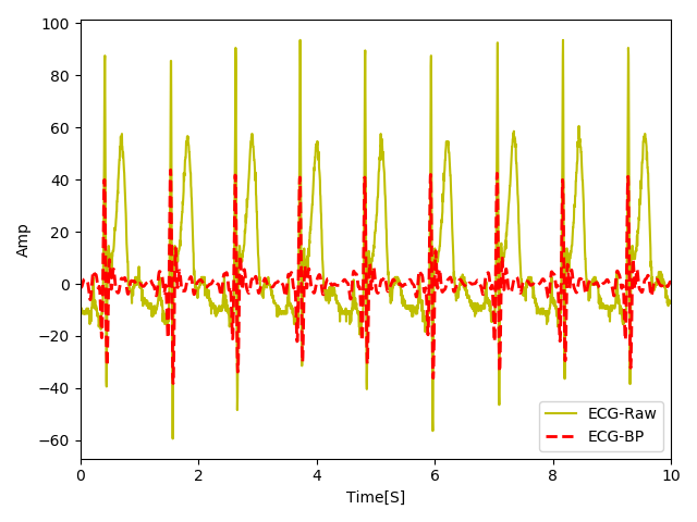
As you can see the bandpass filter is doing a decent job in canceling the frequencies below 5 Hz such as the T-waves which in this signal are highly elevated. This is important because our detector might worngly detect the T-waves as the R wave. Also, the high frequency noise (spikes > 15 hz) is nicely attenuated. Now that we have bandlimited our signal, let's go ahead and see how we can further enhance the R peaks.
2. Differentiation and Squaring:
Probably you remember the term differentiation from your college time. Hopefully, you remember that in order to calculate the slope of a function we can do the following:
Usually signals are sampled with a fixed rate (, where is the sampling frequency), therefore the denominator of the equation above stays constant. Now, the nominator of the equation above increases as the difference between the amplitude of the two consecutive samples increase. Therefore, in order to highlight the sharper peaks in the signal (such as the R peaks), it might be useful to see where the slope is higher. Let’s implement a simple single point differentiator that squares the signal. The reason that we square the signal after the differentation is to further highlight the sharper edges.
def Differentiate(ECG):
    '''
    Compute single difference of the signal ECG
    '''
    ECG_df  = np.diff(ECG)
    ECG_sq  = np.power(ECG_df,2)
    return np.insert(ECG_sq,0, ECG_sq[0])
The function above, simply computes a single point difference in the signal and squares it:
ECG_df = Differentiate(ECG_BP)
ts_df = Series(np.squeeze(ECG_df[:10*Fs]), index=np.arange(ECG_raw[:10*Fs].shape[0])/Fs)
fig = plt.figure(frameon="False"); ts_df.plot(style='r--', label='ECG-differentiate',linewidth=2.0);
ts_BP.plot(style='y',label='ECG-BP')
plt.ylabel('Amp'); plt.xlabel('Time[S]',); plt.legend()
plt.tight_layout(); plt.show()
fig.savefig('ECG_df.png', transparent=True)
In order to make the length of the output signal equal to the input, we simply repeat the first input.
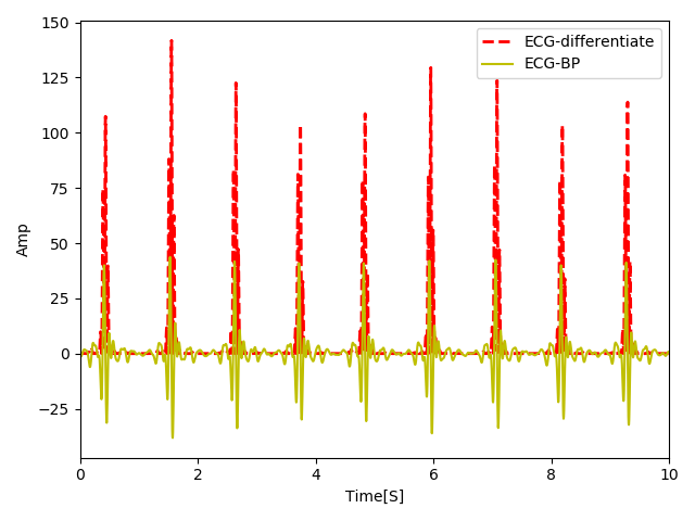
As you can see the smoother edges are attenuated and the sharper are highlighted in the difference and squared signal. The reason that we squared the signal was to further highlight the sharper edges so that the R peaks are easier to detect. However, there is still a problem. After squaring Q and S waves around R are also sharp peaks that might cause our peak detector to wrongly detect them. We will see how we can solve this issue in the next step.
3. Moving Average Window:
As we mentioned before, our output signal from the previous step still contains sharp edges that makes the QRS detection difficult. In this last processing step we apply a simple moving average window that merges these nearby peaks and further cancels out the sharper edges. We can implement a simple moving average in time-domain by convolving a rectangular window with the signal.
def MovingAverage(ECG,N=30):
    '''
    Compute moving average of signal ECG with a rectangular window of N
    '''
    window  = np.ones((1,N))/N
    ECG_ma  = np.convolve(np.squeeze(ECG),np.squeeze(window))
    return ECG_ma
In case, you are curious what we did mathematically,
where, is our input signal with length and is our moving window with length and computed as:
Note that here I chose a moving average window of size 30 points that for the sampling frequency of 250 Hz in this signal seems appropriate. If you increase or decrease the sampling frequency, you may want to tune this value acordingly or make it a function of the sampling rate. This is known as full way of performing the convolution where each overlap is considered. Let’s see how the output signal looks like after this phase.
ECG_ma = MovingAverage(ECG_df)
ts_ma = Series(np.squeeze(ECG_ma[:10*Fs]), index=np.arange(ECG_raw[:10*Fs].shape[0])/Fs)
fig = plt.figure(frameon="False"); ts_df.plot(style='y',label='ECG-DF')
ts_ma.plot(style='r--', label='ECG-MA',linewidth=2.0)
plt.ylabel('Amp'); plt.xlabel('Time[S]',); plt.legend()
plt.tight_layout(); plt.show()
fig.savefig('ECG_ma.png', transparent=True)
Below you see the output of the signal after it is passed through the moving average signal.
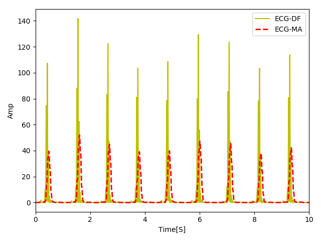
You can see that now our signal looks like a set of smooth mountains. Note that due to convolution we used here, our signal has a phase shift but it is linear in this case, so we could simply shift the signal if required. Finally, we only need to run a peak detector to identify the QRS peaks.
4. Peak Detection and Thresholding:
I promise this is the last stage of our algorithm, just bear with me a little bit more. Now that we have properly rejected unwanted noise and enhanced the signal, we can apply our peak detector. For simplicity, we are going to use the find_peaks function in scipy package. The function below implements our peak detector.
def QRSpeaks(ECG,Fs):
    '''
    Finds peaks in a smoothed signal ECG and sampling freq Fs.
    '''
    peaks, _  = signal.find_peaks(ECG, height=np.mean(ECG), distance=round(Fs*0.200))
    return peaks
In this function, we simply set a threshold equal to the mean of the signal which seems to work quite well. Of course, you could try out different threshold values for yourself (e.g. ) to see how the perfromance changes. In signal processing, we normally tune the threshold by looking at the Receiver Operator Curves (ROC). I will talk more about that in a future post. Finally, note that we have set a minimum distance of 200 msec between each QRS peak since it is physiologically impossible to have two consecutive QRS peaks closer than 200 msec.
QRS = QRSpeaks(ECG_ma,Fs)
QRS = QRS[QRS<=10*Fs]
fig = plt.figure(frameon="False")
plt.plot(np.arange(ECG_raw[:10*Fs].shape[0])/Fs,ECG_raw[:10*Fs],color='y',label='ECG')
plt.vlines(x=(QRS-15)/Fs,ymin=np.min(ECG_raw[:10*Fs]),ymax=np.max(ECG_raw[:10*Fs]),linestyles='dashed',color='r', label='QRS',linewidth=2.0)
plt.ylabel('Amp'); plt.xlabel('Time[S]'); plt.legend()
plt.tight_layout(); plt.show()
fig.savefig('QRS_pks.png', transparent=True)
If you are reading this congratualtions! You just built up your first QRS detector in a short time. See the results of your QRS detector below.
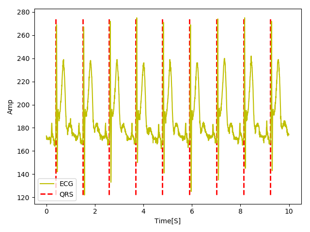
Not bad at all for a simple QRS detector. Here, we plot only the first 10 seconds of the signal but go ahead and plot the whole signal and see for yourself that the detector performs quiet well. It is interesting to note that all the steps I implemented here stem from Pan-Tompkin's paper which dates back to 1985. Impressive isn't it? Once Pan-Tompkin's developed this algorithm, they did not have access to Python or Matlab to develop it in 30 min as we did now. So, I am always amazed at how the quality of research was high 3 decades ago.
Putting It All Together
For you convenience, I have gathered all of the functions in a single script that you could copy paste and run to reproduce all of the steps, we explained above. Now that you have become familiar with the QRS detection process, I encourage you to check out my BioSigKit Pan-tompkin’s algorithm implementation. Please feel free to drop me an email in case you might have any questions or look to consult me!
If you like what I do and want to support my efforts, please feel free to donate a cup of coffee!
'''
Loads an ECG signal with frequency Fs and detects QRS peaks
Author:  Hooman Sedghamiz, Jan, 2019
%% ============== Licensce ========================================== %%
If you use these modules in any other project, please refer to MIT open-source license.
    MIT License
    Copyright (c) 2019 Hooman Sedghamiz
    Permission is hereby granted, free of charge, to any person obtaining a copy
    of this software and associated documentation files (the "Software"), to deal
    in the Software without restriction, including without limitation the rights
    to use, copy, modify, merge, publish, distribute, sublicense, and/or sell
    copies of the Software, and to permit persons to whom the Software is
    furnished to do so, subject to the following conditions:
    The above copyright notice and this permission notice shall be included in all
    copies or substantial portions of the Software.
% THIS SOFTWARE IS PROVIDED BY THE COPYRIGHT HOLDERS AND CONTRIBUTORS
% "AS IS" AND ANY EXPRESS OR IMPLIED WARRANTIES, INCLUDING, BUT NOT
% LIMITED TO, THE IMPLIED WARRANTIES OF MERCHANTABILITY AND FITNESS
% FOR A PARTICULAR PURPOSE ARE DISCLAIMED. IN NO EVENT SHALL THE COPYRIGHT
% OWNER OR CONTRIBUTORS BE LIABLE FOR ANY DIRECT, INDIRECT, INCIDENTAL,
% SPECIAL, EXEMPLARY, OR CONSEQUENTIAL DAMAGES (INCLUDING, BUT NOT LIMITED
% TO, PROCUREMENT OF SUBSTITUTE GOODS OR SERVICES; LOSS OF USE, DATA, OR
% PROFITS; OR BUSINESS INTERRUPTION) HOWEVER CAUSED AND ON ANY THEORY OF
% LIABILITY, WHETHER IN CONTRACT, STRICT LIABILITY, OR TORT (INCLUDING
% NEGLIGENCE OR OTHERWISE) ARISING IN ANY WAY OUT OF THE USE OF THIS
% SOFTWARE, EVEN IF ADVISED OF THE POSSIBILITY OF SUCH DAMAGE.
'''
#-------------- Python 3.7 ------------------#
# Lets import loadmat required to import .mat files
from scipy.io import loadmat
# Of course we also need signal from Scipy too
from scipy import signal
# Importing numpy to make it possible to perform vector operations
import numpy as np
# These two libraries are for visualization
import matplotlib.pyplot as plt
from pandas import Series


def BandPassECG(Path,Fs):
    '''
    This function takes in a "path" and imports the ECG signal in .mat format
    '''
    # Import the signal
    ECG    = loadmat(Path)['EKG5']
    # Implementing the Butterworth BP filter
    W1     = 5*2/Fs                                    # --> 5 Hz cutt-off (high-pass) and Normalize by Sample Rate
    W2     = 15*2/Fs                                   # --> 15 Hz cutt-off (low-pass) and Normalize by Sample Rate
    b, a   = signal.butter(4, [W1,W2], 'bandpass')     # --> create b,a coefficients , since this is IIR we need both b and a coefficients
    ECG    = np.asarray(ECG)                           # --> let's convert the ECG to a numpy array, this makes it possible to perform vector operations
    ECG    = np.squeeze(ECG)                           # --> squeeze
    ECG_BP = signal.filtfilt(b,a,ECG)    # --> filtering: note we use a filtfilt that compensates for the delay
    return ECG_BP,ECG

def Differentiate(ECG):
    '''
    Compute single difference of the signal ECG
    '''
    ECG_df  = np.diff(ECG)
    ECG_sq  = np.power(ECG_df,2)
    return np.insert(ECG_sq,0, ECG_sq[0])

def MovingAverage(ECG,N=30):
    '''
    Compute moving average of signal ECG with a rectangular window of N
    '''
    window  = np.ones((1,N))/N
    ECG_ma  = np.convolve(np.squeeze(ECG),np.squeeze(window))
    return ECG_ma

def QRSpeaks(ECG,Fs):
    '''
    Finds peaks in a smoothed signal ECG and sampling freq Fs.
    '''
    peaks, _  = signal.find_peaks(ECG, height=np.mean(ECG), distance=round(Fs*0.200))
    return peaks

# Load and BP the Signal
Fs =250
Path ='C:/Users/hooman.sedghamiz/Downloads/BioSigKit-master/BioSigKit-master/SampleSignals/ECG5'

# BP Filter
ECG_BP,ECG_raw = BandPassECG(Path,Fs)

# Difference Filter
ECG_df = Differentiate(ECG_BP)

# Moving Average
ECG_ma = MovingAverage(ECG_df)

# QRS peaks
QRS = QRSpeaks(ECG_ma,Fs)

# Plots
fig = plt.figure(frameon="False")
plt.plot(np.arange(ECG_raw.shape[0])/Fs,ECG_raw,color='y',label='ECG')
plt.vlines(x=(QRS-15)/Fs,ymin=np.min(ECG_raw),ymax=np.max(ECG_raw),linestyles='dashed',color='r', label='QRS',linewidth=2.0)
plt.ylabel('Amp'); plt.xlabel('Time[S]'); plt.legend()
plt.tight_layout(); plt.show()
fig.savefig('QRS_pks.png', transparent=True)
Disclaimer
None of the scripts or software provided in this webpage are suitable for any sort of medical diagnosis.